---
title: "Hierarchical Prior Predictive Analysis"
subtitle: "Foundational Report 10"
description: |
Prior predictive validation of the h_m01 hierarchical model at the
alignment-study factorial scale (J=18 cells from a 6×3 design).
Establishes the tightened priors and verifies that implied cell-level
sensitivities, choice distributions, and SEU-maximizer rates are
scientifically plausible.
categories: [foundations, validation, h_m01]
execute:
cache: true
---
```{python}
#| label: setup
#| include: false
import sys
import os
import json
import tempfile
import warnings
warnings.filterwarnings('ignore')
sys.path.insert(0, os.path.join(os.getcwd(), '..'))
project_root = os.path.dirname(os.path.dirname(os.getcwd()))
sys.path.insert(0, project_root)
import numpy as np
import pandas as pd
import matplotlib.pyplot as plt
from IPython.display import Image
np.random.seed(42)
```
## Introduction
[Report 9](09_hierarchical_implementation.qmd) described the Stan implementation of the hierarchical `h_m01` model. Before fitting the model to real alignment-study data we repeat, at the hierarchical scale, the prior-predictive validation we performed for `m_0` in [Report 3](03_prior_analysis.qmd).
The questions are the same in spirit:
1. **Prior validation**: Do the chosen hyperpriors produce sensible *cell-level* sensitivities?
2. **Model understanding**: What range of behaviours is a priori plausible across the 18 experimental cells?
3. **Experimental design**: Is the `6 × 3` factorial rich enough to distinguish the regression effects of interest?
::: {.callout-note}
## The Hierarchical Prior Predictive Distribution
The prior predictive distribution for `h_m01` is induced by:
1. Drawing population hyperparameters: $\gamma_0 \sim \mathcal{N}(2.5, 0.5)$, $\boldsymbol{\gamma} \sim \mathcal{N}(0, 0.5)$, $\sigma_{\text{cell}} \sim \text{half-}\mathcal{N}(0, 0.3)$, $\boldsymbol{\beta}_j \sim \mathcal{N}(0, 1)$, $\boldsymbol{\delta} \sim \text{Dirichlet}(1)$.
2. Deriving cell-level sensitivities via the non-centred parameterisation $\log\alpha_j = \gamma_0 + \mathbf{x}_j^\top \boldsymbol{\gamma} + \sigma_{\text{cell}}\, z_{\alpha,j}$.
3. Computing the choice probabilities $\chi_{j,m}$ for every problem in every cell.
4. Simulating choices $y_{j,m} \sim \text{Categorical}(\chi_{j,m})$.
This gives a joint distribution over (i) population-level effects, (ii) cell-level sensitivities, (iii) per-cell $\boldsymbol{\beta}$-matrices, and (iv) choice behaviours — *before* conditioning on any observed data.
:::
## Study Design: The Alignment Factorial
All hierarchical validation reports use the same design: the `6 × 3` factorial that will be applied in the alignment study, treatment-coded relative to a reference cell.
```{python}
#| label: design-summary
#| echo: true
from utils.study_design_hierarchical import HierarchicalStudyDesign

# Factors: factor 0 = LLM (6 levels), factor 1 = prompt style (3 levels)
# Reference cell (index 0): first LLM × first prompt
X, labels, cell_levels = HierarchicalStudyDesign.treatment_design_matrix(
    factors=[6, 3], reference_indices=[0, 0]
)

print(f"J (cells) = {X.shape[0]}")
print(f"P (regression columns, treatment-coded) = {X.shape[1]}")
print(f"Column labels: {labels}")
print(f"Design-matrix rank: {np.linalg.matrix_rank(X)} "
      f"(= P, so the regression is identified)")
print(f"\nFirst 6 rows of X (cells 0..5, i.e. LLM 0 × prompt 0..2, "
      f"LLM 1 × prompt 0..2):")
print(X[:6])
```
::: {.callout-note}
## Treatment Coding Convention
With `factors=[6, 3]` and `reference_indices=[0, 0]`, the reference cell is
(LLM₀, prompt₀). The implicit intercept is absorbed by $\gamma_0$; the seven
treatment dummies in $\mathbf{x}_j$ toggle on for each non-reference level of
each factor. Therefore $\gamma_0$ = log-sensitivity of the reference cell;
$\gamma_1,\ldots,\gamma_5$ = LLM main effects; $\gamma_6, \gamma_7$ = prompt
main effects. Cells are ordered in Kronecker / row-major form (last factor
varies fastest).
:::
The prior predictive analysis was executed via
`scripts/run_hierarchical_prior_predictive.py` when run from the command
line; inside this report we run the same analysis programmatically with the
tightened priors and the `6 × 3` factorial. Results are cached to disk by
Quarto so the analysis re-runs only when this report changes.
```{python}
#| label: run-prior-predictive
#| output: false
from analysis.hierarchical_prior_predictive import HierarchicalPriorPredictiveAnalysis

# Build the factorial design (J=18, P=7, treatment-coded).
study = HierarchicalStudyDesign.from_factorial(
    factors=[6, 3],
    reference_indices=[0, 0],
    K=3, D=2, R=10, M_per_cell=20,
    min_alts_per_problem=2, max_alts_per_problem=4,
    feature_dist="normal", feature_params={"loc": 0, "scale": 1},
    design_name="h_m01_prior_analysis",
)
study.generate()

# Tightened hyperparameters established in Report 9.
hyperparams = {
    "gamma0_mean": 2.5,
    "gamma0_sd": 0.5,
    "gamma_sd": 0.5,
    "sigma_cell_sd": 0.3,
    "beta_sd": 1.0,
}

output_dir = tempfile.mkdtemp(prefix="h_m01_prior_")

analysis = HierarchicalPriorPredictiveAnalysis(
    study_design=study,
    output_dir=output_dir,
    n_param_samples=200,
    n_choice_samples=5,
    hyperparams=hyperparams,
)
_ = analysis.run()

def _img(path, width=720):
    """Display a PNG from the prior-predictive output directory."""
    return Image(filename=os.path.join(output_dir, path), width=width)
```
```{python}
#| label: load-summary
#| echo: false
summary = json.load(open(os.path.join(output_dir, "summary.json")))
hp = summary["hyperparameters"]
print("Hyperparameters used:")
for k, v in hp.items():
print(f" {k} = {v}")
print(f"\nDimensions: J={summary['J']}, P={summary['P']}, "
f"K={summary['K']}, D={summary['D']}, R={summary['R']}, "
f"M_total={summary['M_total']}")
```
## Prior Distributions of the Hyperparameters
### Grand log-sensitivity $\gamma_0$ and cell-level noise $\sigma_{\text{cell}}$
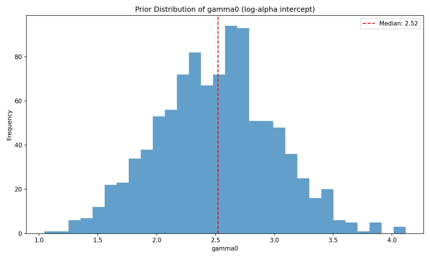
`gamma0` is the log-sensitivity of the reference cell. The tightened prior
$\mathcal{N}(2.5, 0.5)$ places 95 % of its mass on $\gamma_0 \in [1.5, 3.5]$,
corresponding to a reference-cell sensitivity $\alpha_{\text{ref}} \in [4.5,
33]$ — a scientifically reasonable range for "moderately rational" agents.
```{python}
#| label: fig-gamma0-prior
#| fig-cap: "Prior distribution of $\\gamma_0$ from the simulation block of h_m01_sim.stan."
_img("regression_parameters/gamma0_dist.png")
```
```{python}
#| label: fig-sigma-prior
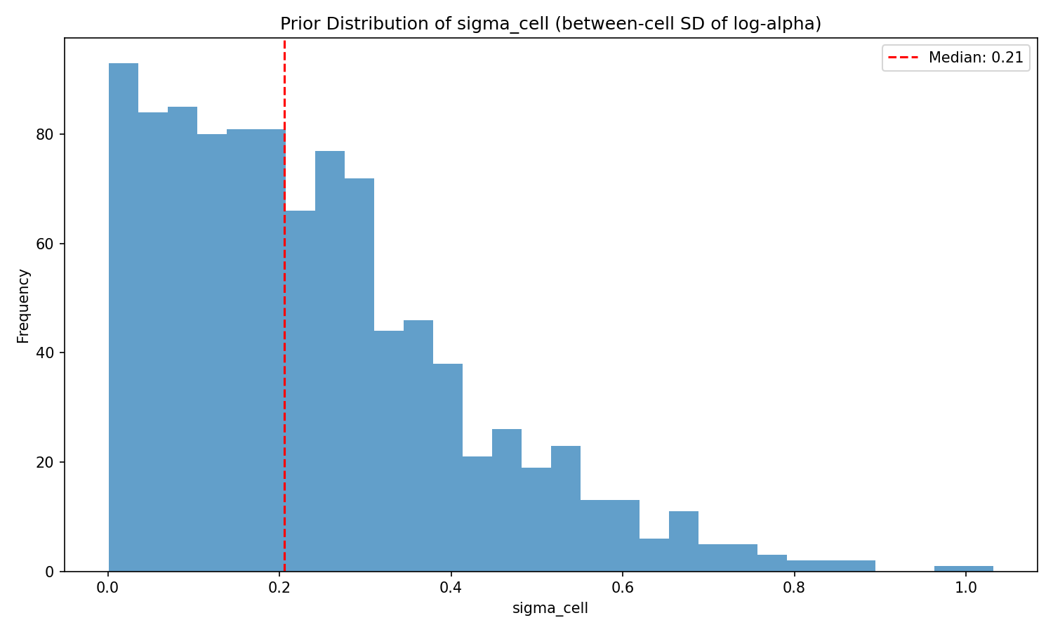
#| fig-cap: "Prior distribution of the cell-level noise SD $\\sigma_\\text{cell}$. The half-normal(0, 0.3) keeps the cell-level deviations modest — 95th percentile $\\approx 0.59$ — so that unexplained between-cell variation in $\\log\\alpha$ does not swamp the regression signal."
_img("regression_parameters/sigma_cell_dist.png")
```
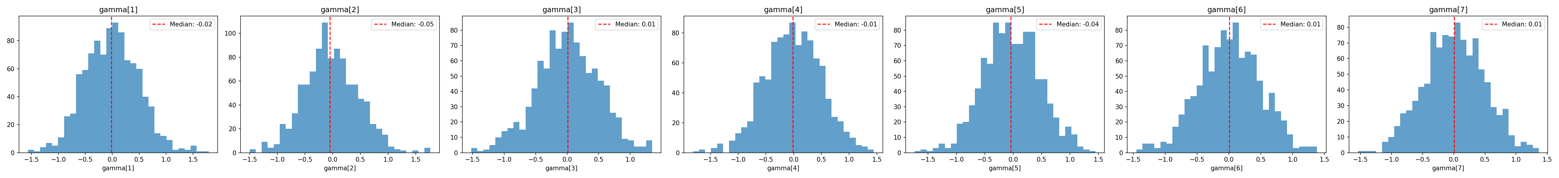
### Regression coefficients $\boldsymbol{\gamma}$
Each of the seven treatment dummies is given $\mathcal{N}(0, 0.5)$ independently. On the log-$\alpha$ scale, a single coefficient of $0.5$ corresponds to a ~65 % multiplicative increase in $\alpha$ for cells where the dummy is on (and a coefficient of $-0.5$ to a ~40 % decrease).
```{python}
#| label: fig-gamma-prior
#| fig-cap: "Prior distributions of the seven regression coefficients $\\gamma_1,\\ldots,\\gamma_7$."
_img("regression_parameters/gamma_dist.png")
```
```{python}
#| label: gamma-prior-stats
#| echo: false
gamma_keys = [k for k in summary["parameter_summary"] if k.startswith("gamma")]
rows = []
for k in gamma_keys:
s = summary["parameter_summary"][k]
rows.append([k, round(s["mean"], 3), round(s["std"], 3),
round(s["q05"], 3), round(s["q95"], 3)])
df = pd.DataFrame(rows, columns=["param", "mean", "sd", "q05", "q95"])
df.to_string(index=False)
```
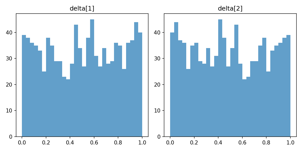
### Utility simplex $\boldsymbol{\delta}$
The symmetric Dirichlet(1) prior keeps the shared utility increments $\boldsymbol{\delta}$ uniform on the simplex, matching the convention of the flat model ([Report 3](03_prior_analysis.qmd)).
```{python}
#| label: fig-delta-prior
#| fig-cap: "Prior on $\\boldsymbol{\\delta}$ (left) and the induced utilities $\\boldsymbol{\\upsilon}$ (right)."
_img("utilities/delta_dist.png")
```
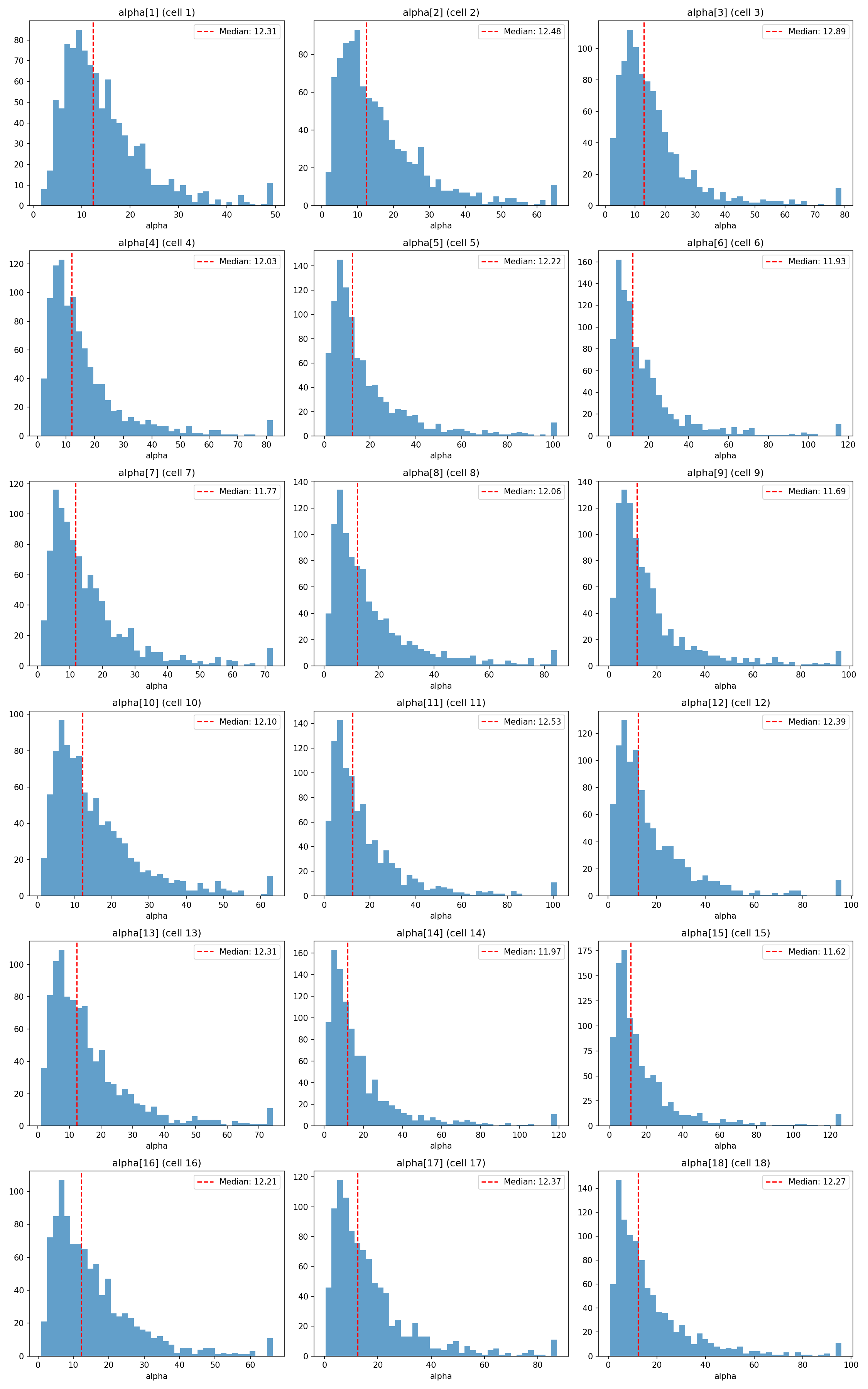
## Prior Distributions over Cell-Level Sensitivities $\boldsymbol{\alpha}$
The real scientific object in `h_m01` is the vector of cell-level sensitivities. A priori each $\alpha_j$ is approximately lognormal around $e^{\gamma_0} \approx 12$, stretched by the regression effects and cell-level noise.
```{python}
#| label: fig-alpha-by-cell
#| fig-cap: "Prior distribution of cell-level $\\alpha_j$ for each of the 18 cells. Dispersion across cells reflects the combined effect of the seven regression dummies and of $\\sigma_\\text{cell}$."
_img("cell_alphas/alpha_by_cell.png")
```
```{python}
#| label: alpha-prior-stats
#| echo: false
alpha_keys = [f"alpha[{j+1}]" for j in range(summary["J"])]
rows = []
for k in alpha_keys:
s = summary["parameter_summary"][k]
rows.append([k, round(s["median"], 2), round(s["q05"], 2),
round(s["q95"], 2), round(s["mean"], 2), round(s["std"], 2)])
df = pd.DataFrame(
rows, columns=["cell", "median", "q05", "q95", "mean", "sd"]
)
print("Summary of prior marginals for cell-level α (tail quantiles "
"in log-normal units):\n")
print(df.to_string(index=False))
```
Key features:
- **Medians** are tightly clustered at $11.6$–$12.9$ across all 18 cells — the cells differ in a priori centrality only modestly, as intended given $\boldsymbol{\gamma} \sim \mathcal{N}(0, 0.5)$.
- **95 th percentiles** stay in the $30$–$60$ range; no cell's prior spills into the "hyper-sharp" regime ($\alpha > 100$) where the softmax saturates. This is the key difference from the original, wider priors — under which the upper prior tail routinely exceeded $140$ and induced divergent transitions during sampling (see [Report 11](11_hierarchical_parameter_recovery.qmd)).
- **90 % intervals** are comfortably bounded, covering the behaviourally meaningful range from weak-to-strong SEU sensitivity without advocating either near-random or deterministic choice.
## Prior-Predictive Choice Behaviour
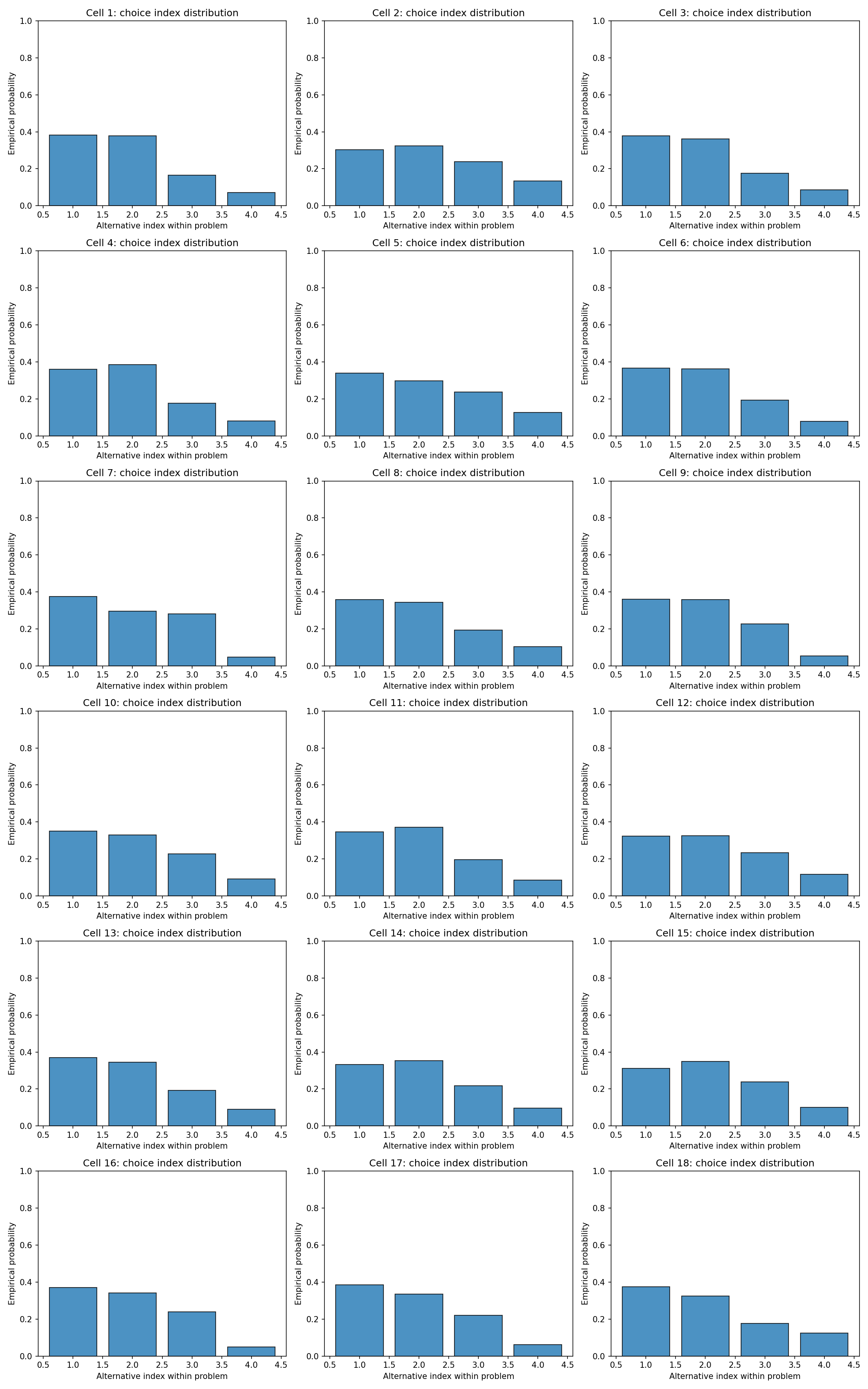
### Chosen-alternative distributions
For each parameter draw we simulated $R = 10$ choices per cell. Aggregating across draws and cells, the prior predicts a balanced but not uniform spread over the shared alternatives, with moderate concentration on the alternatives that happen to dominate the SEU ordering in a given draw.
```{python}
#| label: fig-choice-by-cell
#| fig-cap: "Distribution of choice indices across the 18 cells under the prior predictive. Each row is a cell; columns are the (within-problem) alternative indices."
_img("choices/choice_index_by_cell.png")
```
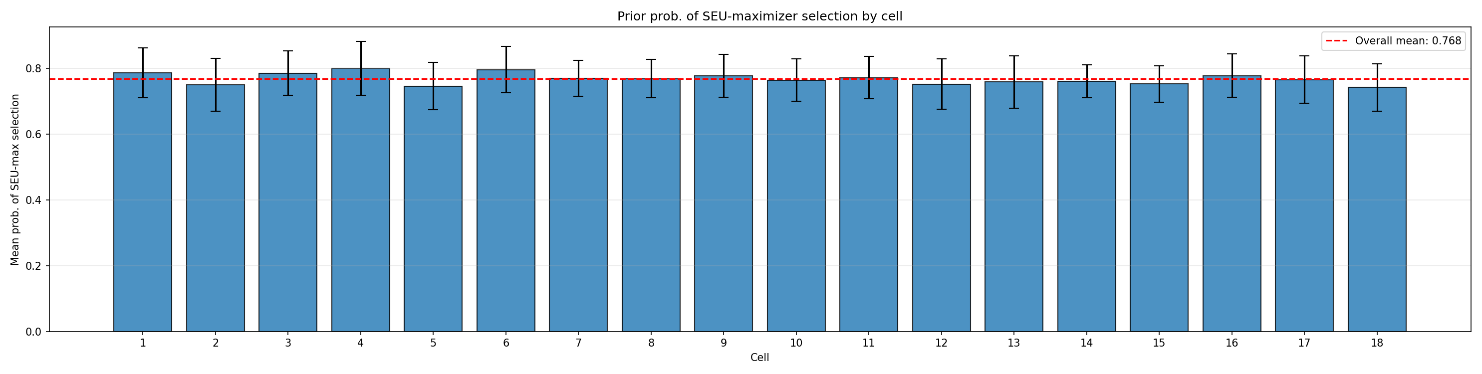
### SEU-maximiser selection rates
A particularly interpretable summary is the **probability that the chosen alternative is the SEU-maximiser** for its problem — i.e. whether the agent acts optimally under its own beliefs and utilities. Under the tightened priors:
```{python}
#| label: seu-max-summary
#| echo: false
seu = json.load(open(os.path.join(
output_dir, "seu_maximizer_selection", "seu_maximizer_summary.json")))
print(f"Overall P(SEU-maximiser selected) = "
f"{seu['overall_prob_seu_max']:.3f}")
print(f"Problems analysed: {seu['total_problems']}")
print(f"Total SEU-max selected per simulation: mean="
f"{seu['total_seu_max_selected']['mean']:.1f}, "
f"sd={seu['total_seu_max_selected']['std']:.1f} "
f"(out of {seu['total_problems']})")
print("\nPer-cell mean P(SEU-maximiser):")
for j in range(1, 19):
cell = seu["prob_seu_max_by_cell"][str(j)]
print(f" cell {j:>2}: mean={cell['mean']:.3f}, "
f"sd={cell['std']:.3f}")
```
```{python}
#| label: fig-seu-max-by-cell
#| fig-cap: "Per-cell prior probability that the SEU-maximiser is chosen."
_img("seu_maximizer_selection/prob_seu_max_by_cell.png")
```
The overall rate (~0.77) sits in the intended middle range: high enough to make genuine SEU-maximising behaviour the modal outcome, low enough to leave substantial room for sub-optimal (and, in the alignment context, *super-optimal*) treatment effects to be detected.
::: {.callout-tip}
## Scientific Interpretation
A prior that concentrated P(SEU-max) near 1.0 would be too committed to optimality — the posterior would struggle to update toward "this LLM is noisy" without a great deal of data. A prior that placed P(SEU-max) near $1/|\text{alts}| \approx 0.3$ would be effectively uninformative about rationality. The tightened priors leave the *entire* alignment-relevant range identifiable.
:::
## Comparison with the Pre-Tightening Priors
The original `h_m01` defaults were $\gamma_0 \sim \mathcal{N}(3, 1)$, $\boldsymbol{\gamma} \sim \mathcal{N}(0, 1)$, $\sigma_{\text{cell}} \sim \text{half-}\mathcal{N}(0, 0.5)$, and $\boldsymbol{\beta} \sim \mathcal{N}(0, 1)$. Under those priors the 97.5 th percentile of the prior predictive for $\alpha$ frequently exceeded $140$, pushing the softmax into near-deterministic regimes where the likelihood flattens and posterior exploration becomes unstable. The tightened priors (used throughout this and subsequent reports) preserve the scientifically meaningful range while restoring sampler geometry to a regime where HMC can operate reliably.
::: {.callout-note}
## Provenance and Reproducibility
This report runs `HierarchicalPriorPredictiveAnalysis` live on every build
(Quarto caches the result so it re-runs only when the report itself
changes). The same analysis can be reproduced from the command line via
```bash
python scripts/run_hierarchical_prior_predictive.py \
    --config configs/h_m01_prior_analysis_config.json
```
The design uses `factors=[6, 3]` and `reference_indices=[0, 0]` (treatment
coding), giving $J = 18$ cells and $P = 7$ regression columns.
:::
```{python}
#| label: cleanup
#| include: false
import shutil
try:
shutil.rmtree(output_dir)
except Exception:
pass
```
## Summary
The hierarchical prior predictive analysis establishes three things:
1. **Cell-level sensitivities are well-behaved**: $\alpha_j$ medians cluster near 12 across cells, with 95th percentiles below 60 — avoiding the flat-likelihood regime that caused pathological sampling under the original priors.
2. **Implied choice behaviour is scientifically reasonable**: the overall SEU-maximiser selection rate ≈ 0.77 leaves room for both sub-optimal and super-optimal treatment effects to be detected.
3. **The treatment-coded design is identified**: $\mathbf{X}$ has full column rank 7, with $\gamma_0$ plus five LLM dummies and two prompt dummies forming an orthogonal main-effects parameterisation of the $6 \times 3$ factorial.
[Report 11](11_hierarchical_parameter_recovery.qmd) takes the next step: can we *recover* the known hyperparameters when we simulate data from this prior and fit `h_m01` back to it?