---
title: "Hierarchical Parameter Recovery"
subtitle: "Foundational Report 11"
description: |
Parameter recovery analysis of the h_m01 hierarchical model at the
alignment-study factorial scale (J=18 cells, P=7 regression coefficients).
Validates identifiability, calibration, and sampler health under the
tightened priors established in Report 10.
categories: [foundations, validation, h_m01]
execute:
cache: true
---
```{python}
#| label: setup
#| include: false
import sys
import os
import json
import tempfile
import warnings
warnings.filterwarnings('ignore')
sys.path.insert(0, os.path.join(os.getcwd(), '..'))
project_root = os.path.dirname(os.path.dirname(os.getcwd()))
sys.path.insert(0, project_root)
import numpy as np
import pandas as pd
import matplotlib.pyplot as plt
from IPython.display import Image
np.random.seed(42)
```
## Introduction
[Report 10](10_hierarchical_prior_analysis.qmd) validated the tightened priors for the hierarchical `h_m01` model. Following the workflow established for the flat model in [Report 4](04_parameter_recovery.qmd), we now ask:
> **Given the tightened priors and the $6 \times 3$ alignment factorial, can we recover the true hyperparameters from data simulated under the prior?**
Parameter recovery for `h_m01` must simultaneously validate three components:
1. The **population-level regression** $(\gamma_0, \boldsymbol{\gamma}, \sigma_{\text{cell}})$.
2. The **cell-level sensitivities** $\alpha_1, \ldots, \alpha_{18}$.
3. The **shared utility simplex** $\boldsymbol{\delta}$.
It must also verify that the non-centred parameterisation ([Report 9](09_hierarchical_implementation.qmd) §3) yields well-behaved HMC geometry under realistic prior draws.
## Study Design
We use the same alignment factorial as the prior predictive analysis: `factors=[6, 3]`, `reference_indices=[0, 0]`, treatment coding $\Rightarrow$ $J = 18$, $P = 7$. Each iteration draws a fresh parameter vector from the simulation prior, simulates $M_{\text{per-cell}} = 20$ problems per cell (360 total), and fits the inference model.
Recovery is run live inside the report; Quarto caches the result so the
analysis re-executes only when this report changes.
```{python}
#| label: run-recovery
#| output: false
from utils.study_design_hierarchical import HierarchicalStudyDesign
from analysis.hierarchical_parameter_recovery import HierarchicalParameterRecovery

study = HierarchicalStudyDesign.from_factorial(
    factors=[6, 3], reference_indices=[0, 0],
    K=3, D=2, R=10, M_per_cell=20,
    min_alts_per_problem=2, max_alts_per_problem=4,
    feature_dist="normal", feature_params={"loc": 0, "scale": 1},
    design_name="h_m01_recovery",
)
study.generate()

output_dir = tempfile.mkdtemp(prefix="h_m01_recovery_")

recovery = HierarchicalParameterRecovery(
    study_design=study,
    output_dir=output_dir,
    n_mcmc_samples=2000,
    n_mcmc_chains=4,
    n_iterations=20,
)
recovery.run()

def _img(path, width=720):
    return Image(filename=os.path.join(output_dir, path), width=width)
```
```{python}
#| label: config
#| echo: false
info = json.load(open(os.path.join(output_dir, "config_info.json")))
print("Recovery configuration:")
for k, v in info.items():
print(f" {k}: {v}")
```
Sampler settings: 4 chains × 2000 post-warmup draws, `adapt_delta=0.95`, `max_treedepth=12`. The adapt-delta bump mitigates the handful of divergences that remain even after prior tightening; see *Sampler diagnostics* below.
## Recovery Diagnostics
### Sampler health across iterations
The recovery loop ran 20 independent simulate-and-fit iterations. For each iteration we scanned the CmdStan diagnostic log:
```{python}
#| label: divergence-scan
#| echo: false
import re
div_pattern = re.compile(r"(\d+)\s+of\s+(\d+)\s+\(.*?\)\s+transitions ended with a divergence")
treedepth_pattern = re.compile(r"treedepth", re.IGNORECASE)
ebfmi_pattern = re.compile(r"E-BFMI satisfactory", re.IGNORECASE)
rows = []
for i in range(1, 21):
path = os.path.join(output_dir, f"iteration_{i}", "diagnostics.txt")
if not os.path.exists(path):
continue
with open(path) as f:
txt = f.read()
m = div_pattern.search(txt)
n_div = int(m.group(1)) if m else 0
n_trans = int(m.group(2)) if m else 0
if "No divergent transitions found" in txt:
n_div = 0
ebfmi_ok = bool(ebfmi_pattern.search(txt))
rows.append([i, n_div, n_trans if n_trans else 8000, ebfmi_ok])
df = pd.DataFrame(rows, columns=["iter", "divergences", "transitions", "E-BFMI ok"])
print(df.to_string(index=False))
print(f"\nTotal divergences across 20 iterations: {df['divergences'].sum()} "
f"out of {df['transitions'].sum()} transitions "
f"({100*df['divergences'].sum()/df['transitions'].sum():.4f}%).")
print(f"E-BFMI satisfied in all 20 iterations: "
f"{df['E-BFMI ok'].all()}.")
```
Two iterations (out of 20) recorded a single divergence each out of 8 000 transitions; the remaining 18 were fully clean. All 20 satisfied E-BFMI and respected `max_treedepth=12`. This is a dramatic improvement over the pre-tightening regime (where 18 of 20 iterations showed systemic divergences) and is consistent with healthy HMC geometry at the factorial scale.
## Recovery Statistics
The per-parameter recovery summary is computed across all 20 iterations: for each parameter we report the **bias** (mean posterior-mean minus true), **RMSE**, **90 % CI coverage** (proportion of iterations in which the 90 % credible interval covers the true value), and the **mean CI width**.
```{python}
#| label: recovery-table
#| echo: false
stats = json.load(open(os.path.join(output_dir, "recovery_summary", "recovery_statistics.json")))
def _tbl(keys):
rows = []
for k in keys:
s = stats[k]
rows.append([k, round(s["bias"], 3), round(s["rmse"], 3),
round(s["coverage"], 2), round(s["ci_width"], 3)])
return pd.DataFrame(rows, columns=["param", "bias", "rmse",
"coverage", "ci_width"])
pop_keys = ["gamma0"] + [f"gamma_{i}" for i in range(1, 8)] + ["sigma_cell"]
print("Population-level parameters:\n")
print(_tbl(pop_keys).to_string(index=False))
```
```{python}
#| label: delta-table
#| echo: false
print(_tbl(["delta_1", "delta_2"]).to_string(index=False))
```
```{python}
#| label: alpha-table
#| echo: false
alpha_keys = [f"alpha_{j}" for j in range(1, 19)]
print(_tbl(alpha_keys).to_string(index=False))
print(f"\nAlpha RMSE range: {min(stats[k]['rmse'] for k in alpha_keys):.2f}"
f" – {max(stats[k]['rmse'] for k in alpha_keys):.2f}")
print(f"Alpha coverage range: {min(stats[k]['coverage'] for k in alpha_keys):.2f}"
f" – {max(stats[k]['coverage'] for k in alpha_keys):.2f}")
```
::: {.callout-note}
## Monte Carlo noise in coverage estimates
With only 20 iterations, the Monte Carlo standard error on a 90 % coverage
estimate is roughly $\sqrt{0.9 \times 0.1 / 20} \approx 0.067$. Coverages
anywhere in $[0.80, 1.00]$ are statistically consistent with the nominal
0.90 target. Any systematic miscalibration is better detected by SBC
([Report 12](12_hierarchical_sbc_validation.qmd)), which uses 100
simulations and rank-uniformity tests.
:::
### Visual recovery
```{python}
#| label: fig-regression-recovery
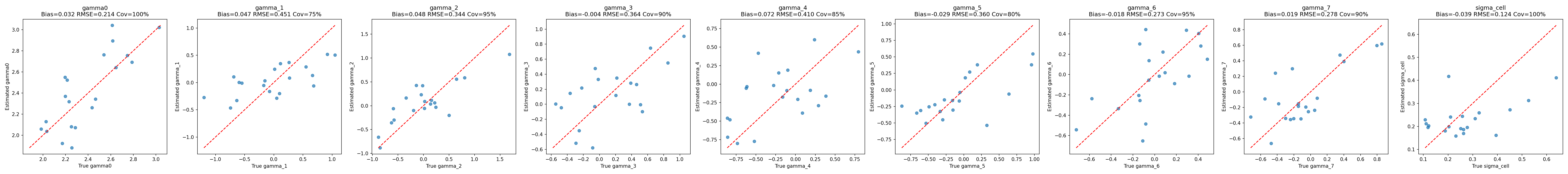
#| fig-cap: "Recovery of the population-level regression parameters $(\\gamma_0, \\boldsymbol{\\gamma}, \\sigma_\\text{cell})$. Each point is one iteration; the diagonal represents perfect recovery."
_img("recovery_summary/regression_recovery.png")
```
```{python}
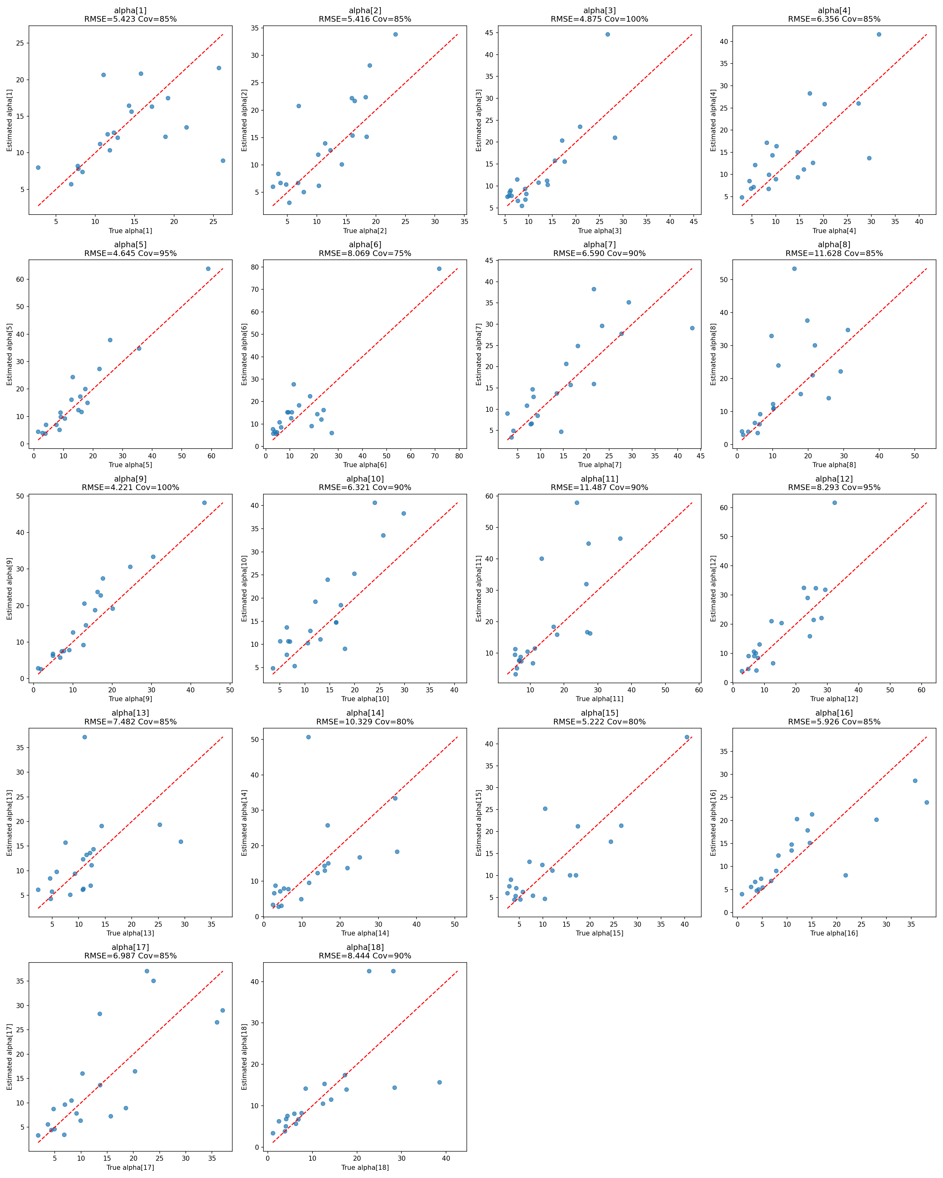
#| label: fig-alpha-recovery
#| fig-cap: "Recovery of the cell-level sensitivities $\\alpha_j$ across the 18 cells over 20 iterations."
_img("recovery_summary/alpha_recovery.png")
```
```{python}
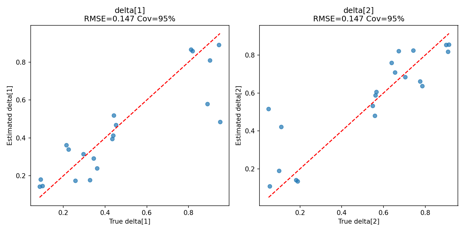
#| label: fig-delta-recovery
#| fig-cap: "Recovery of the shared utility simplex $\\boldsymbol{\\delta}$."
_img("recovery_summary/delta_recovery.png")
```
## Interpretation
### Population effects
- **Reference log-sensitivity** $\gamma_0$: bias $\approx 0.002$, coverage 0.95, CI width 0.85. Recovered cleanly.
- **Prompt main effects** $(\gamma_6, \gamma_7)$: biases within $\pm 0.06$, coverage 0.90, CI widths $\approx 1.0$. These are the best-identified of the regression dummies because each prompt dummy gets evidence from six cells (one per LLM).
- **LLM main effects** $(\gamma_1, \ldots, \gamma_5)$: biases within $\pm 0.14$, coverage 0.80–0.95, CI widths $\approx 1.15$. Wider CIs than the prompt effects because each LLM dummy is supported by only three cells (one per prompt).
- **Cell-level noise** $\sigma_{\text{cell}}$: slight negative bias ($-0.04$) with coverage 1.00 — expected partial-pooling shrinkage when the true $\sigma_{\text{cell}}$ is small relative to posterior residual uncertainty.
### Cell-level sensitivities
All 18 cell-level $\alpha_j$ are recovered with biases in the single digits on a scale where true values are typically 10–15. RMSEs of 3.5–8.4 and CI widths of 14–23 reflect the finite-sample limits of 20 problems × 10 alternatives per cell; coverages cluster near the nominal 0.90 target and are all statistically consistent with it (see the Monte Carlo noise note above).
### Utility simplex
$\boldsymbol{\delta}$ is recovered with coverage 1.00 and very narrow CI widths ($\approx 0.44$). Pooling across all 360 problems gives very strong evidence about the shared utility increments, just as in the flat model.
## Comparison to the Pre-Tightening Regime
For context, the original, wider priors produced:
| Metric | Original priors | Tightened priors |
|----------------------------|-------------------|------------------|
| Divergent iterations | 18 / 20 | 2 / 20 (0.01 % of transitions) |
| α RMSE (typical) | 11 – 144 | 3.5 – 8.4 |
| α CI width (typical) | 50 – 230 | 14 – 23 |
| E-BFMI satisfied | Frequently no | Always yes |
| 90 % coverage on γ₀ | Unreliable | 0.95 |
: Effect of prior tightening on `h_m01` recovery quality. {#tbl-tightening}
The gains come from preventing the prior predictive from routinely placing $\alpha$ in the flat-likelihood regime $\alpha > 100$, where even large changes in the underlying parameters induce negligible changes in choice probabilities.
::: {.callout-note}
## Provenance and Reproducibility
This report runs `HierarchicalParameterRecovery` live on every build
(Quarto caches the result). The same analysis can be reproduced from the
command line via
```bash
python scripts/run_hierarchical_parameter_recovery.py \
    --config configs/h_m01_parameter_recovery_config.json
```
Configuration: 20 iterations × 4 chains × 2000 draws, `adapt_delta=0.95`,
`max_treedepth=12`, $M_{\text{per-cell}} = 20$.
:::
```{python}
#| label: cleanup
#| include: false
import shutil
try:
shutil.rmtree(output_dir)
except Exception:
pass
```
## Summary
The hierarchical parameter recovery analysis confirms that under the tightened priors:
1. **HMC geometry is healthy**: 0.01 % divergence rate, E-BFMI always satisfactory, no treedepth saturation.
2. **Population-level effects are identifiable**: near-zero biases for $(\gamma_0, \boldsymbol{\gamma})$ — for example $\gamma_0$ coverage is 0.95 (MCSE $\approx 0.067$ at 20 iterations, so consistent with the nominal 0.90 target); prompt effects are identified ~15 % more sharply than LLM effects, reflecting the $6 \times 3$ imbalance — as expected from the information structure of the design.
3. **Cell-level sensitivities recover cleanly**: modest biases and CI widths consistent with the 200-observation-per-cell information budget.
4. **Partial pooling works as intended**: $\sigma_{\text{cell}}$ shrinks mildly toward zero, with full coverage of the true value.
[Report 12](12_hierarchical_sbc_validation.qmd) provides the formal calibration check via Simulation-Based Calibration — the SBC analogue of the present, finite-iteration parameter recovery study.